From Words to Vectors: Understanding Tokens and Embeddings in Modern LLMs

As we already know, computers operate at a low level using 0s and 1s, which are numerical values that can represent text, images, audio, or video. AI models are no different: if you expect a model to understand a raw sentence with no numeric representation, that assumption is wrong. So, how does an AI model turn text into numerical representations it can process?

TL;DR

• Tokenization splits text into identifiable units and maps them to IDs

• Embeddings turn those IDs into learned vectors that models can compare and process

Remember: AI does not read words

You might argue with the statement “AI does not read words.” After all, when we type a question into ChatGPT, Gemini, or Claude, the chatbot responds in natural language. It feels like the model is reading and understanding words the way we do. Not exactly.

I typed this statement “When the front door opened, I saw someone I never expected” into ChatGPT. It responded with a short story continuing from my prompt text and wrapped it up like a little fairy tale.

How does it do that? Behind the scenes, the model is performing math. That leads to the real question: how does a model turn a sentence into a response if it only performs math?

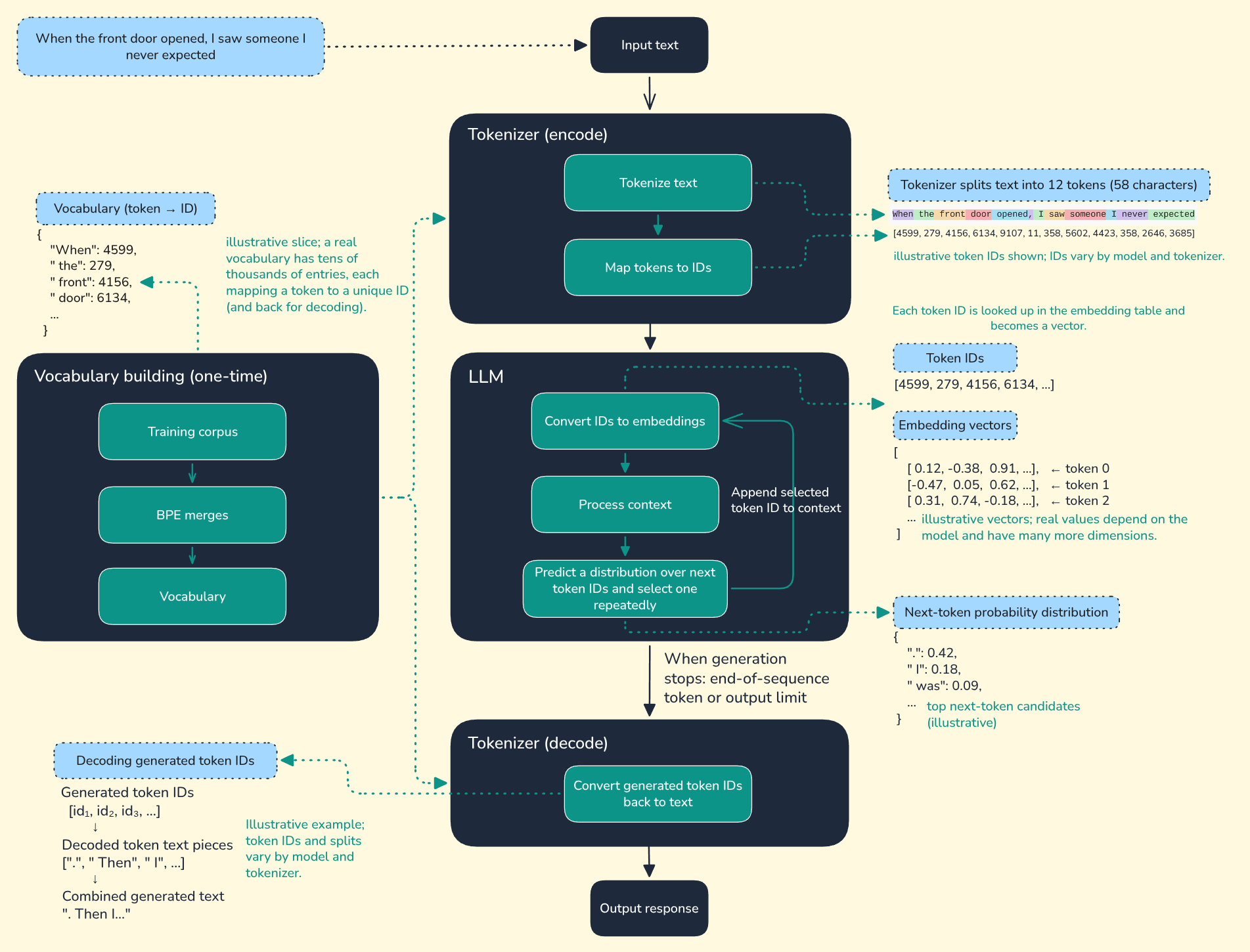
This post focuses on tokenization and the embedding stage: building the vocabulary, splitting text into tokens, mapping them to IDs, and turning IDs into vectors. The LLM processing, next-token prediction, and decoding are shown for context and covered in later posts.

To answer all of these questions, I’m going to break it down into two parts.

Part 1: From Text to Vectors

Before an LLM can process text, a tokenizer splits it into tokens and maps each token to a token ID. An embedding layer then maps those IDs to vectors.

Step 1: Text is split into tokens

What is a token in the context of an LLM?

A token is a piece of text, such as part of a word, a whole word, punctuation, or a space depending on the tokenizer.

Say, I have a sentence cats chase cats. If you run it through the OpenAI Tokenizer, this sentence splits into 3 tokens (15 characters): cats chase cats.

Note: The “4 Characters” Rule of Thumb: one token is roughly 4 characters or 0.75 words (or 100 tokens ≈ 75 words). This can vary by tokenizer, model, language, and input type. This average is specific to common English text. In other languages (especially non-Latin scripts) or programming code, a single token might represent far fewer characters.

Let’s see a simple example of a tokenizer to get the idea:

text = "cats chase cats"

tokens = text.split()    # ["cats", "chase", "cats"]

# text -> tokens

Three tokenization strategies

• Word-level tokenization treats each word as a token. It struggles with typos and previously unseen words.

• Character-level tokenization treats every character as a token. It can represent any text, but produces long sequences.

• Subword tokenization splits text into recurring pieces between full words and characters. It is common in modern LLMs because it keeps the vocabulary manageable while representing unfamiliar words with known pieces.

After tokenization, the model operates on token IDs rather than the visible token text. However, tokens are not conceptually discarded: they are the vocabulary units that connect text to token IDs and allow generated IDs to be decoded back into text.

Step 2: How a tokenizer builds its vocabulary

Vocabulary is a key part of tokenization because it connects tokens to their token IDs. Before getting to how real tokenizers build one, let’s extend our cats chase cats example to build a simple vocabulary.

vocab = {token: i for i, token in enumerate(sorted(set(tokens)))}

print(vocab)    # {'cats': 0, 'chase': 1}

# tokens -> vocabulary

Subword tokenizers don’t build their vocabulary by listing whole words like our example did. They learn it from a large training corpus with an algorithm. The most common subword algorithms are Byte-Pair Encoding (BPE), WordPiece, and Unigram; we’ll focus on BPE.

BPE works in rounds. It starts from individual characters, counts every adjacent pair across the corpus, merges the single most frequent pair into a new token, and repeats until the vocabulary reaches a target size. A single word can’t show this, since the merges are driven by frequency across many words, so let’s run it on a small corpus (each word with its count):

"cat" ×9   "cap" ×4   "car" ×6   "can" ×11   "scan" ×3

Here is BPE running on that corpus. Each word starts split into characters, and the most frequent adjacent pair is merged each round:

import collections

# Training corpus: word -> frequency. Each word starts as space-separated characters.
corpus = {"c a t": 9, "c a p": 4, "c a r": 6, "c a n": 11, "s c a n": 3}

def count_pairs(corpus):
    pairs = collections.Counter()
    for word, freq in corpus.items():
        symbols = word.split()
        for a, b in zip(symbols, symbols[1:]):
            pairs[(a, b)] += freq
    return pairs

def merge_pair(pair, corpus):
    bigram, merged = " ".join(pair), "".join(pair)
    return {word.replace(bigram, merged): freq for word, freq in corpus.items()}

for step in range(3):
    pairs = count_pairs(corpus)
    best = max(pairs, key=pairs.get)    # most frequent adjacent pair
    print(f"round {step+1}: merge {best} -> '{''.join(best)}'")
    corpus = merge_pair(best, corpus)

print("final:", corpus)

Output:

round 1: merge ('c', 'a') -> 'ca'
round 2: merge ('ca', 'n') -> 'can'
round 3: merge ('ca', 't') -> 'cat'
final: {'cat': 9, 'ca p': 4, 'ca r': 6, 'can': 11, 's can': 3}

How did it choose those merges? Each round counts every adjacent pair across the corpus and merges the most frequent one. In round 1:

(c, a) is the most frequent (it appears in every word), so it merges into a new token ca. Rounds 2 and 3 then recount and merge the next winners, ca + n becomes can and ca + t becomes cat, exactly as the output shows.

These merge rules are saved in order. At runtime the tokenizer replays them, so a frequent word like cat becomes a single token, while an unseen word like cats still decomposes into known pieces (cat + s) instead of failing. That is how subword tokenization keeps the vocabulary small while still covering words it never saw during training.

This is a minimal illustration; production BPE adds details like deterministic tie-breaking and word-boundary handling (the simple str.replace here works because this tiny corpus has no overlapping or repeated pairs within a word).

Step 3: Tokens become IDs, but IDs have no meaning by themselves

When a tokenizer function splits text into tokens, it also maps each token to a numeric token ID.

Continue building on the example above from Steps 1 and 2:

token_ids = [vocab[token] for token in tokens]

print(token_ids)    # [0, 1, 0]

# tokens -> vocabulary -> token IDs

If we combine the code, the output is:

['cats', 'chase', 'cats']
{'cats': 0, 'chase': 1}
[0, 1, 0]

[0, 1, 0] is the sequence of identifiers for ["cats", "chase", "cats"] from the example text above. They’re not a “meaning score” and IDs differ across model tokenizers.

The .split() example above is just for intuition. Notice the leading spaces in my inline example, cats chase cats: real tokenizers treat cats and cats as different tokens, because the space is encoded as part of the token. Production LLMs use trained subword tokenizers that work this way. Let’s inspect one with the tiktoken library:

import tiktoken

text = "cats chase cats"

for name in ["cl100k_base", "o200k_base"]:
    enc = tiktoken.get_encoding(name)    # cl100k_base: GPT-3.5-turbo/GPT-4 family; o200k_base: GPT-4o family
    ids = enc.encode(text)
    pieces = [enc.decode([i]) for i in ids]
    print(name, ids)
    print("       ", pieces)

Output:

cl100k_base [38552, 33586, 19987]
        ['cats', ' chase', ' cats']
o200k_base [70782, 59591, 28854]
        ['cats', ' chase', ' cats']

Two things to notice. First, the text splits into the same three tokens in both tokenizers, and the leading spaces ( cats, not cats) are part of the token. Second, the token IDs are different (38552 vs 70782 for cats, 19987 vs 28854 for cats). The ID is just an index into that specific tokenizer’s vocabulary, so the same word gets different IDs across models. This is exactly why you must use a model’s own tokenizer to count its tokens.

Some may ask: why do tokens matter? Tokens matter for two reasons. First, they make text computable. Second, their count determines how much text fits in the model’s context window, which affects cost, processing speed, and response limits.

Step 4: IDs become embeddings

Now you have a better understanding of tokens and token IDs.

What is an embedding?

An embedding is a learned vector of floating-point numbers that represents the meaning or features of an item, such as a token, word, sentence, image, or document.

The following code shows how the model looks up an embedding for each token ID.

import numpy as np

# A tiny vocabulary: token -> ID
vocab = {
    "cat": 0,
    "dog": 1,
    "car": 2,
}

# A learned embedding table in a real model.
# These values are manually chosen here only for illustration.
embedding_table = np.array([
	[0.9, 0.8, 0.1],    # cat
	[0.8, 0.9, 0.1],    # dog
	[0.1, 0.2, 0.9],    # car
])

# Function to calculate cosine similarity between two vectors
def cosine_similarity(vector_a, vector_b):
	return np.dot(vector_a, vector_b) / (
	    np.linalg.norm(vector_a) * np.linalg.norm(vector_b)
    )

cat_vector = embedding_table[vocab["cat"]]
dog_vector = embedding_table[vocab["dog"]]
car_vector = embedding_table[vocab["car"]]

print("cat embedding:", cat_vector)
print("cat vs dog:", round(cosine_similarity(cat_vector, dog_vector), 2))
print("cat vs car:", round(cosine_similarity(cat_vector, car_vector), 2))

Expected result: cat is more similar to dog than to car.

cat embedding: [0.9 0.8 0.1]
cat vs dog: 0.99
cat vs car: 0.3

In a real model, embedding vectors are not manually assigned. They are learned and adjusted during training from patterns in large amounts of data.

An embedding table is a matrix with V rows (one for every token in the vocabulary) and d columns (the dimensions of each embedding vector). Looking up a token ID selects one row.

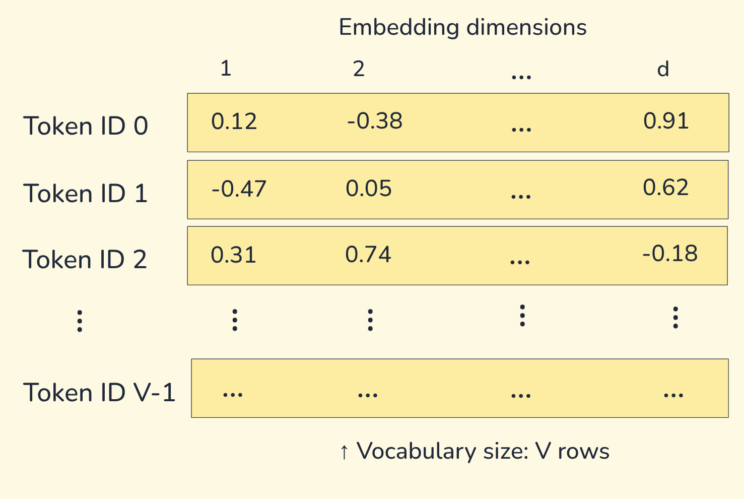
vocabulary size × embedding dimension = V × d

Each token ID selects one row from this matrix. That row is the token’s embedding vector.

For example, if a tokenizer has 100,000 tokens and each embedding has 768 numbers, its embedding table has shape: 100,000 × 768.

At first glance, a list of token IDs and an embedding vector can both look like arrays of numbers. However, they serve different roles. A token ID is an integer that identifies a token in a tokenizer’s vocabulary. For example, an ID such as 38552 is simply a dictionary key; its numerical value does not tell us anything about the token’s meaning.

An embedding, on the other hand, is the learned vector selected by that token ID from the embedding table. Unlike the ID, the embedding contains many floating-point values that the neural network can use to represent patterns and relationships learned during training.

In short, a token ID answers, “Which vocabulary entry is this?” An embedding answers, “What numerical representation should the model use for this entry?”

Note: The embedding looked up here is the same every time for a given token ID. It does not yet account for surrounding words. How a model adjusts these vectors based on context is a separate topic I’ll cover when we get to Transformers.

Part 2: Understanding and Using Embeddings

Once text is represented as vectors, we can compare those vectors and use them in tasks such as semantic search, recommendations, and clustering.

Cosine similarity: measuring vector similarity

The embedding vectors in the above example are deliberately chosen so that cat is more similar to dog than to car. In a real model, this relationship is learned from training data and the model’s training objective.

Cosine similarity is a common way to compare embedding vectors. It compares their directions: a higher score means the vectors point in more similar directions; a lower score means the vectors are less directionally aligned.

Similarity is useful for finding related patterns, but it is not a guarantee that two items have the same meaning or that a result is factually correct. For example, cat and dog may have a high similarity score because they are related animals, but they are not the same thing. Embedding similarity reflects learned patterns in training data, not literal equality or factual verification.

Token embeddings and text embeddings are different

Token embeddings and text embeddings are related, but they are not the same thing. Both begin with tokenized text, but a token embedding represents each individual token as a vector. A text or document embedding represents an entire piece of text as one vector.

• A token embedding represents one token from a model’s vocabulary.

• A text or document embedding represents an entire sentence, paragraph, or document.

Text embeddings support semantic search, recommendations, clustering, and Retrieval-Augmented Generation (RAG). For example, a semantic-search system can retrieve a note about tokenization for the query: “How do LLMs split text?”

Try it yourself

1. Use the OpenAI Tokenizer to compare token counts for an English sentence, a code snippet, and a non-English phrase. Token counts vary by model and tokenizer, so the same text may split differently in other tools or models.

2. Change the vectors in the example embedding table and observe how the cosine-similarity scores change.

Conclusion

Tokens and embeddings form the bridge between human text and machine computation. Tokenization decides how text is split and identified; embeddings turn those identifiers into learned vectors that allow models to compare patterns and similarity.

With these foundations in place, we can better understand how LLMs turn text into numerical representations. I will continue exploring and documenting the concepts that build on this process.

References

• OpenAI Tokenizer

• What are tokens and how to count them

• Tokenization algorithm guide

• Words to Vectors

• OpenAI: Vector Embeddings

• Stanford CS224N: Word Vectors lecture

• Hugging Face: Semantic search with FAISS