Neural Networks from First Principles: A Beginner’s Guide

In my last post, I mentioned going deeper into neural networks, the core foundation of today’s modern deep learning. But, before diving into the details, we first need to understand the concept.

What is a neural network?

Imagine a human brain: a network of billions of neurons, each linked to thousands of others through trillions of connections. Pretty amazing, right? An artificial neural network is a simplified mathematical imitation of that idea: neurons passing signals to other neurons. Its mechanism is to learn patterns from example data without rules written by a human.

Neural networks are used for various tasks such as pattern recognition, classification, weather forecasting, fraud detection, predictive analytics and more. Several things we use daily are built on neural networks without us realizing it. Think of face or fingerprint unlock on your phone, spam detection in email, Amazon product recommendations, Netflix’s “what to watch next”, and many other applications.

The idea goes back further than you’d think. The first mathematical model of a neuron came from Warren McCulloch and Walter Pitts in 1943. What’s changed since is the data and computing power that finally let these decades-old ideas take off. To me, Artificial Intelligence (AI) is the most influential and fastest-growing industry I’ve ever seen. Models like ChatGPT, Claude, Gemini, and Qwen, plus many open-weight versions, keep coming out constantly, each improving on the last. They’re incredibly powerful now, yet they still produce mistakes and hallucinations. That’s exactly why it’s worth understanding what’s happening underneath. That is what this post is about.

Under the hood

AI is the broader field that includes machine learning. Deep learning is a major part of machine learning, and neural networks are the core tool behind deep learning. Each level builds on the previous one. A neural network itself has multiple layers and a process flow that computes before producing the final output.

I will show you just a few points to memorize as it’s easier to learn little by little than throwing the whole thing in all at once.

Let’s focus on its layers and process flow.

Layers

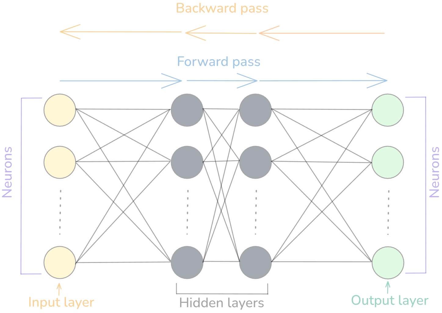
The simplest way to understand a neural network is as three types of layers: input, hidden, and output. These are the fundamental and core layers for a neural network to learn.

The process flows from one end to the other and produces an output. Each layer is a group of nodes connected to the nodes in the next layer. The node is called an artificial neuron. Each neuron receives inputs through weights, adds a bias, then applies an activation function. It computes and produces an activation value representing how strongly a pattern is detected. Some activations, like sigmoid, squeeze that value between 0 and 1; others, like ReLU, can output larger values, but those are not covered in this post.

Process Flow

In the figure above, it looks like the signal flows left to right, but the direction isn’t really the point. It’s just one way to picture data moving from one end to the other: input layer → hidden layer → output layer. Each flow from one neuron to the other neuron is triggered by a small piece of math: a weighted sum plus a bias.

z = w \cdot x + b

That is the equation of a straight line: the weight $w$ scales the input $x$ , and the bias $b$ shifts it. Here’s the catch that matters later: stacking straight lines on top of each other still gives you a straight line. For example, feed $y = 2 x + 1$ into $z = 3 y + 4$ and it collapses to $z = 6 x + 7$ , one line again. That’s why a network needs the “bend” from the activation function in point 3 below.

Beyond that, if you think of it as a mathematical pattern, it’s hard to grasp without getting into calculus and linear algebra. The simplest way is to think of it as pattern-matching that is learned and refined over and over, with each neuron passing an activation value to the next layer.

The forward pass makes a prediction, but learning happens through the full training loop: predict, measure the loss, send error information backward with backpropagation, then update the weights and biases. Backpropagation is an algorithm used to train the network by applying the principle of error correction. First, the loss function measures how wrong the network is (the difference between the predicted output and the true output). Backpropagation then sends that error backward through the network to work out how much each weight and bias contributed to it. Finally, those weights and biases are nudged in the direction that reduces the error, improving accuracy over many rounds.

The figure below shows one full training cycle, from prediction to error to weight update, repeated over and over.

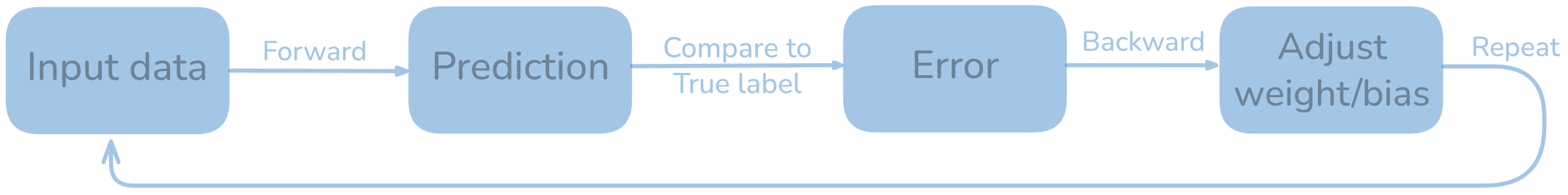
This process takes a lot of computation, and how much depends on the input data and the chain of operations involved. If it’s not done right, the model ends up performing poorly.

5 Essential Principles a Neural Network Can’t Live Without

As you already know, a neural network can learn from the data and make predictions. But, how does it do that, and what makes it learn, and what is the process? These are the questions people just starting to explore AI for the first time always ask.

To answer these questions, I’ll take a simple example: a study-hours classifier, and then go through piece by piece with the math and real code examples shown alongside each other.

Given input $x$ (hours studied), it predicts output $y$ (pass or fail).

1. Input Data

A neural network learns from data. If there is no input data, there is nothing to learn. This is the most fundamental. The same principle applies to us: if we’ve never seen or known a cat before, we wouldn’t be able to identify it as a cat. So, sample data of cats is important for the network to learn.

To demonstrate this, let’s write the math for an input example:

x = [x_1,x_2,x_3,x_4,x_5]

y = [y_1,y_2,y_3,y_4,y_5]

Assuming hours of study is an array $x$ which contains hours of 1, 2, 3, 4, 5 and $y$ is the actual output presented as pass/fail: 1 is pass and 0 is fail. If a student studies for 1 or 2 hours, he/she would fail. At 3 hours or more, they would pass.

x=[1,2,3,4,5]

y = [0,0,1,1,1]

Written in Python code should be:

x = np.array(1],[2],[3],[4],[5)
y = np.array(0],[0],[1],[1],[1)

2. Weights & Biases

Think of the weight as how much something matters, and the bias as a starting offset. In our study example, $x$ is the hours studied, the weight $w$ decides how much each hour pushes the score up, and the bias $b$ shifts the result up or down regardless of the input. Multiply the input by its weight and add the bias, and you get $z$ , the neuron’s raw score before any activation.

z=w \cdot x + b

Here we have a single input, so $z$ is just $w \cdot x + b$ . With more inputs, each gets its own weight and you add them all up, a weighted sum: $z = w_{1} x_{1} + w_{2} x_{2} + \dots + b$ .

So if a student studies 4 hours, each hour is worth 0.5, and the baseline is 0.1:

$x = 4$
$w = 0.5$
$b = 0.1$

The result should be:

$z = 0.5 \times 4 + 0.1$
$z = 2.1$

Written in Python code should be:

x = 4
w = 0.5
b = 0.1

z = w * x + b

3. Activation Function (Non-linear)

As I mentioned above, a linear function combined with another linear function is still linear, so the network can’t learn complex patterns. Picture trying to separate dots arranged in a ring from dots in the middle. No straight line can do it. Linear transformations on their own can only draw straight-line boundaries, and stacking only linear transformations still gives you another linear transformation. The activation function lets the network bend those lines into curves, which is how it learns anything more complex than a straight split. This is the one point that beginners underrate: it’s the reason deep networks can represent complex patterns at all.

Let’s take a look at the sigmoid function, a classic activation function often used for binary classification outputs:

\sigma(z) = \frac{1}{1 + e^{-z}}

Where:

$σ$ (sigma) is the output of the sigmoid function.
$z$ is the input value coming from a neuron.
$e$ is Euler’s number, approximately 2.71828.

Given an example of $z = 2.1$ , the $σ (z)$ is about 0.89.

In a trained binary classifier, a sigmoid output of 0.89 can be interpreted as a high probability-like score for passing.

Written as Python code:

def sigmoid(z):
    return 1 / (1 + np.exp(-z))

y_pred = sigmoid(z)

4. Loss Function

The single “how wrong” number. With no definition of wrong, there’s no direction to improve in. This is called binary cross-entropy (log loss).

For one training example, the loss function is:

L = -\left[y \log(\hat{y}) + (1-y)\log(1-\hat{y})\right]

Where:

$L$ = loss
$y$ = actual answer
$\overset{y}{^}$ = prediction

When the true answer is 1, only the first term matters, so the loss is just $- lo g (\overset{y}{^})$ :

small error: $- lo g (0.89) \approx 0.12$ (barely wrong leads to a tiny loss)
large error: $- lo g (0.05) \approx 3.0$ (confidently wrong leads to a big loss)

That’s the whole point: the more confidently wrong the prediction, the bigger the penalty.

Written in Python code:

epsilon = 1e-9  # keeps log() from blowing up at exactly 0 or 1

loss = -np.mean(
    y * np.log(y_pred + epsilon)
    +
    (1 - y) * np.log(1 - y_pred + epsilon)
)

5. Learning

The mechanism that turns “how wrong” into “which way to nudge each knob.” Without it, the loss just sits there.

A. Backpropagation: calculates the gradients, which answers the question of “how much did each weight contribute to the error?”

The definitions behind weight ( $d w$ ) and bias ( $d b$ ) are:

dw = \frac{\partial L}{\partial w}

db = \frac{\partial L}{\partial b}

Normally, working out $\frac{\partial L}{\partial w}$ means chaining several derivatives together. But because we paired the sigmoid with cross-entropy loss, almost everything cancels out and the error per example collapses to a single clean term: $\overset{y}{^} - y$ . So the gradients become:

dw = \frac{1}{N}\,x^{\top}(\hat{y}-y)

db = \text{mean}(\hat{y}-y)

which is exactly what the code computes:

error = y_pred - y
dw = (x.T @ error) / len(x)
db = np.mean(error)

B. Gradient Descent (Optimizer): uses gradients to update parameters. The gradient points in the direction that makes the error larger, so we step the opposite way (that’s the minus sign) to go downhill. The learning rate controls step size: too big and you overshoot, too small and learning crawls.

Math definition of a new weight and a new bias:

w_{\text{new}} = w_{\text{old}} - \alpha \frac{\partial L}{\partial w}

b_{\text{new}} = b_{\text{old}} - \alpha \frac{\partial L}{\partial b}

Where:

$α$ = learning rate

Written in Python code should be:

w = w - learning_rate * dw
b = b - learning_rate * db

A real example:
old weight = 0.50
gradient = 0.50
learning rate = 0.10
new weight = 0.45

Now let’s put all five pieces together into one tiny working program: a single-neuron classifier, the simplest version of the neural network idea.

import numpy as np


# -----------------------------
# 1. Input data
# -----------------------------
# x = study hours
x = np.array([
    [1.0],
    [2.0],
    [3.0],
    [4.0],
    [5.0],
])

# y = pass/fail
# 0 = fail, 1 = pass
y = np.array([
    [0.0],
    [0.0],
    [1.0],
    [1.0],
    [1.0],
])


# -----------------------------
# 2. Initialize weights
# -----------------------------
np.random.seed(42)

w = np.random.randn(1, 1)
b = np.zeros((1, 1))


# -----------------------------
# 3. Activation function
# -----------------------------
def sigmoid(z):
    return 1 / (1 + np.exp(-z))


# -----------------------------
# 4. Loss function
# -----------------------------
def binary_cross_entropy(y_true, y_pred):
    epsilon = 1e-9

    loss = -np.mean(
        y_true * np.log(y_pred + epsilon)
        + (1 - y_true) * np.log(1 - y_pred + epsilon)
    )

    return loss


# -----------------------------
# 5. Training loop
# -----------------------------
learning_rate = 0.1
epochs = 5000

for epoch in range(epochs):
    # Forward pass
    z = x @ w + b
    
    # Activation
    y_pred = sigmoid(z)

    # Calculate loss
    loss = binary_cross_entropy(y, y_pred)

    # Backpropagation
    error = y_pred - y

    dw = (x.T @ error) / len(x)
    db = np.mean(error)

    # Optimizer: update weights/biases
    w = w - learning_rate * dw
    b = b - learning_rate * db

    # Print progress occasionally
    if epoch % 500 == 0:
        print(f"Epoch {epoch}, Loss: {loss:.4f}")


# -----------------------------
# Final learned parameters
# -----------------------------
print("\nFinal weight:", w)
print("Final bias:", b)

Output result

Epoch 0, Loss: 0.5385
Epoch 500, Loss: 0.1907
Epoch 1000, Loss: 0.1317
Epoch 1500, Loss: 0.1044
Epoch 2000, Loss: 0.0877
Epoch 2500, Loss: 0.0761
Epoch 3000, Loss: 0.0674
Epoch 3500, Loss: 0.0606
Epoch 4000, Loss: 0.0551
Epoch 4500, Loss: 0.0505

Final weight: [[4.24834391]]
Final bias: [[-10.41946338]]

To test the prediction using the final weight and bias, we should have this:

# -----------------------------
# Test predictions
# -----------------------------
test_x = np.array([
    [1.5],
    [2.5],
    [3.5],
    [6.0],
])

z = test_x @ w + b
predictions = sigmoid(z)

print("\nPredictions:")
for hours, prediction in zip(test_x, predictions):
    print(f"{hours[0]} study hours → pass probability: {prediction[0]:.4f}")

Output result

Predictions:
1.5 study hours → pass probability: 0.0172
2.5 study hours → pass probability: 0.5502
3.5 study hours → pass probability: 0.9885
6.0 study hours → pass probability: 1.0000

Conclusion

And that’s the simplest neural-network-style model from first principles: one neuron learning a binary decision. We started with five pieces a network can’t live without (data, weights and biases, a non-linear activation, a loss, and an optimizer) and watched them work together on a tiny problem: predicting pass or fail from study hours. The network started out guessing, measured how wrong it was, and nudged its weights over and over until the predictions made sense.

Here’s the part worth sitting with: the giant models behind ChatGPT, Claude, and Gemini build on these same core ideas. They have billions more parameters, far more data, and much more complex architectures, but the core training pattern is the same: predict, measure the error, adjust, repeat. Once you can see it in a small working example, you can see it everywhere.

References

Neural networks by 3Blue1Brown: https://www.youtube.com/watch?v=aircAruvnKk

Gradient Descent by IBM: https://www.youtube.com/watch?v=i62czvwDlsw
Backpropagation by IBM: https://www.youtube.com/watch?v=S5AGN9XfPK4
A Logical Calculus of the Ideas Immanent in Nervous Activity: https://www.cse.chalmers.se/~coquand/AUTOMATA/mcp.pdf
Another Backpropagation introduction: https://visionbook.mit.edu/backpropagation.html